Flow Between Parallel Plates

This section is about the computation and visualization of the velocity and pressure fields in an incompressible fluid between two parallel infinitely large plates using OpenFOAM and ParaView. The results obtained by OpenFOAM are compared to the analytical solutions available for this particular flow case.

Analytical Solution

The fluid is set in motion due to the shear forces caused by the movement of the plates relative to each other. The positions and velocities of the plates are given in Figure 1 with respect to a cartesian coordinate system (x,y,z).

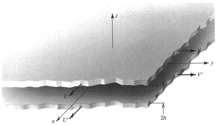
Figure 1: Parallel plates and the cartesian coordinate system [1]

The plates are a distance 2h apart from each other and the coordinate system is centered in the middle of this distance so that the top plate is located at z=h and the bottom plate is located at z=-h. The Navier-Stokes equations describing incompressible fluid flow in x,y,z directions are given below [1]:

x-direction:

\[\frac{\partial u}{\partial t}+u\frac{\partial u}{\partial x}+v\frac{\partial u}{\partial y}+w\frac{\partial u}{\partial z}=-\frac{1}{\rho}\frac{\partial p}{\partial x}+\nu\cdot \Big(\frac{\partial^2 u}{\partial x^2}+\frac{\partial ^2 u}{\partial y^2}+\frac{\partial^2 u}{\partial z^2}\Big)\]

y-direction:

\[\frac{\partial v}{\partial t}+u\frac{\partial v}{\partial x}+v\frac{\partial v}{\partial y}+w\frac{\partial v}{\partial z}=-\frac{1}{\rho}\frac{\partial p}{\partial y}+\nu\cdot \Big(\frac{\partial^2 v}{\partial x^2}+\frac{\partial ^2 v}{\partial y^2}+\frac{\partial^2 v}{\partial z^2}\Big)\]

z-direction:

\[\frac{\partial w}{\partial t}+u\frac{\partial w}{\partial x}+v\frac{\partial w}{\partial y}+w\frac{\partial w}{\partial z}=-g-\frac{1}{\rho}\frac{\partial p}{\partial z}+\nu\cdot \Big(\frac{\partial^2 w}{\partial x^2}+\frac{\partial ^2 w}{\partial y^2}+\frac{\partial^2 w}{\partial z^2}\Big)\]

In the Navier-Stokes equation for the z-direction the g term denotes the gravitational constant. In all equations \(\nu\) is the kinematic viscosity of the fluid, \(p\) is the pressure and \(u,v,w\) are the velocity components in the x,y,z directions respectively. The steady state flow assumption requires the local time derivatives of the velocity components (\(\frac{\partial u}{\partial t}, \frac{\partial v}{\partial t},\frac{\partial w}{\partial t}\)) to be equal to zero. Another assumption is that the pressure changes only in x and z directions. The no-slip boundary conditions are given below:

\[u=U,\quad v=V \quad \text{at z=h}\]

\[u=U',\quad v=V' \quad \text{at z=-h}\]

In order to obtain the velocity profile at an arbitrary point, the velocity components \(u\) and \(v\) are assumed to be functions of z only such that \(\mathbf{v}=u(z)\mathbf{e}_1+v(z)\mathbf{e}_2\) where \(\mathbf{v}\) denotes the velocity vector field and \(\mathbf{e}_1\) and \(\mathbf{e}_2\) denote the unit vectors in x and y directions respectively.

Here is a list of assumptions that we made so far to describe fluid flow between two infinitely large plates moving with respect to each other:

• The flow is parallel to the plates \(\Rightarrow w=0\)
• Steady flow \(\Rightarrow \displaystyle\frac{\partial u}{\partial t}=\displaystyle\frac{\partial v}{\partial t}=\displaystyle\frac{\partial w}{\partial t}=0\)
• \(\displaystyle\frac{\partial p}{\partial y}=0\)
• \(\mathbf{v}=u(z)\mathbf{e}_1+v(z)\mathbf{e}_2\)

The application of the above assumptions to the Navier-Stokes equations yields the following simplified governing equations of fluid motion:

\[\begin{split}\begin{matrix}\text{x-direction:}\\ \text{y-direection:} \\ \text{z-direction:}\end{matrix} \begin{pmatrix}0\\0\\0\end{pmatrix}=\begin{pmatrix}-(1/\rho)\partial_x p+\nu u''\\ \nu v'' \\ -g-(1/\rho)\partial_z p\end{pmatrix}\end{split}\]

or

\[\Big[-\displaystyle\frac{1}{\rho}\partial_x p+\nu u''\Big]\mathbf{e}_1+\Big[\nu v''\Big]\mathbf{e}_2+\Big[-g-\displaystyle\frac{1}{\rho}\partial_z p\Big]\mathbf{e}_3=0\]

In the above equations \(\partial_x\) and \(\partial_z\) stand for the partial derivatives with respect to x and z respectively. By integrating the z-direction simplified Navier-Stokes equation once we obtain:

\[p(x,z)=-g\rho z+f_1(x) \qquad (1)\]

From the above description of \(p(x,z)\) it follows that \(\partial_x p=\partial_x f_1\). Plugging this relationship into the x-direction simplified Navier-Stokes equation we obtain:

\[\rho\nu u''=\partial_x f_1\]

Since in the above equation the left hand side is a function of z only and the right hand side is a function of x only, both the left and the right hand sides must be equal to a constant value such that:

\[\rho \nu u''=\partial_x f_1=\partial_x p=C\]

A second expression for the pressure field can be obtained by integrating the equation \(\partial_x p=C\) with respect to x once. This expression is given in Eq.(2)

\[p(x,z)=Cx+f_2(z) \qquad (2)\]

A comparison of Eq.(1) and Eq.(2) shows that \(f_1(x)=Cx\) and \(f_2(z)=-g\rho z\). Using this, the pressure field can be described as in Eq.(3) where \(p_0\) is the pressure at the point x=0, z=0.

\[\boxed{p(x,z)=Cx-g\rho z + p_0} \qquad (3)\]

Furthermore, integrating the equation \(\rho \nu u''=C\) with respect to z twice, we obtain Eq.(4) which describes the x-component of the velocity field:

\[u(z)=\displaystyle\frac{C}{2\rho\nu}z^2+c_1z+c_2 \qquad (4)\]

Applying the boundary conditions for u at z=-h and at z=h, the constants of integration \(c_1,c_2\) can be computed as in Eq.(5).

\[\boxed{u(z)=\displaystyle\frac{C}{2\rho\nu}z^2+\displaystyle\frac{U-U'}{2h}z+\displaystyle\frac{U+U'}{2}-\displaystyle\frac{Ch^2}{2\rho\nu}}\qquad (5)\]

Similarly, the velocity field in y-direction can be obtained by integrating the equation \(\nu v''=0\) (the Navier-Stokes equation for y-direction) twice with respect to z and using the boundary conditions for v at z=-h and at z=h as in Eq.(6).

\[\boxed{v(z)=\displaystyle\frac{V-V'}{2h}z+\displaystyle\frac{V+V'}{2}}\qquad (6)\]

A sub-class of flow between parallel plates is called Couette flow which occurs when \(\partial_x p=0\) in addition to the assumptions listed previously. In the next section about the simulation in OpenFOAM the Couette flow is demonstrated first. Afterwards the more general case of \(\partial_xp \neq 0\) is demonstrated which is called Poiseuille flow.

In case of Couette flow the application of the condition \(\partial_x p=C=0\) to Eq.(5) results in the following solution for the x-direction velocity and pressure profiles:

\[\begin{split}\text{Couette flow: }\quad u(z)=\displaystyle\frac{U-U'}{2h}z+\displaystyle\frac{U+U'}{2}\qquad (7)\\p(z)=-\rho g z+p_0 \qquad (8)\end{split}\]

Numerical Solution using OpenFOAM

This section contains step-by-step instructions for the pre-processing, solving and post-processing of Couette and Poiseuille flows whose analytical solutions have been derived in the previous section.

Couette Flow

Inside the home/username/OpenFOAM folder create a new folder called Couette. Then, inside the Couette folder create three more folders called 0, constant and system. The 0 folder will contain the initial velocity and pressure conditions, the constant folder will contain the mesh description and material properties and the system folder will contain some solver parameters which will be explained on examples in the subsequent sections.

Definition of the simulation domain and the mesh properties: The Couette flow will be simulated by taking a strip from the infinite fluid between the plates. The long side of this strip is 4 m long in x-direction, its height is equal to 2h=0.2 m and its depth is equal to 0.01 m. The geometry of this finite strip is shown in Figure 2.

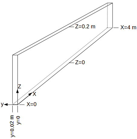
Figure 2: Couette flow simulation domain

In order to discretize the geometry shown in Figure 2, create a new folder called polyMesh inside the constant folder and inside the polyMesh folder create a file called ‘blockMeshDict’. The blockMeshDict file contains the parameters used by the ‘blockMesh’ program in order to generate the finite volume mesh for the geometry discretization. The blockMesh command should be executed in the Linux terminal from within the Couette folder in order to invoke the mesh generation program blockMesh. The following code block shows what the blockMeshDict file should look like.

blockMeshDict file:

/*--------------------------------*- C++ -*----------------------------------*\
| =========                 |                                                 |
| \\      /  F ield         | OpenFOAM: The Open Source CFD Toolbox           |
|  \\    /   O peration     | Version:  2.4.0                                 |
|   \\  /    A nd           | Web:      www.OpenFOAM.org                      |
|    \\/     M anipulation  |                                                 |
\*---------------------------------------------------------------------------*/
FoamFile
{
    version     2.0;
    format      ascii;
    class       dictionary;
    object      blockMeshDict;
}
// * * * * * * * * * * * * * * * * * * * * * * * * * * * * * * * * * * * * * //

convertToMeters 0.01;

vertices
(
    (0 0 0)
    (400 0 0)
    (400 0 20)
    (0 0 20)
    (0 2 0)
    (400 2 0)
    (400 2 20)
    (0 2 20)
);

blocks
(
    hex (0 1 2 3 4 5 6 7) (40 1 20) simpleGrading (1 1 1)
);

edges
(
);

boundary
(
    top
    {
        type wall;
        faces
        (
            (3 7 6 2)
        );
    }
    bottom
    {
        type wall;
        faces
        (
            (1 5 4 0)
        );
    }
    inlet
    {
        type patch;
        faces
        (
            (0 4 7 3)
        );
    }
    outlet
    {
        type patch;
        faces
        (
            (2 6 5 1)
        );
    }
    frontAndBack
    {
        type empty;
        faces
        (
            (0 3 2 1)
            (4 5 6 7)
        );
    }
  );

  mergePatchPairs
  (
  );

The initial part of the above blockMeshDict file up to the convertToMeters command can be copied from one of the sample files that come with the OpenFOAM installation and can be found in the folder home/username/OpenFOAM/FOAM_RUN/tutorials. In the next part of this section the commands in the blockMeshDict file are explained.

Explanation of the blockMeshDict file

convertToMeters: The number that comes after this command is multiplied with the vertex coordinates. The results of this multiplication are stored in the computer memory as the vertex coordinates with respect to the cartesian coordinate system shown in Figure 2 with the unit of meters. For example, if the number that comes after convertToMeters is 0.1 and the x-coordinate of a vertex is defined as 20 in the blockMeshDict file, then the x-coordinate of this vertex is stored in the computer memory as 2 meters away from the origin in x-direction.

vertices: In OpenFOAM the domain of analysis is partitioned into blocks and afterwards for each block a meshing scheme is defined. In this current example since the domain is simple, it can be described using a single block. This block has the shape of a rectangular prism(Figure 2) and it can be defined using the coordinates of its eight vertices. These coordinates are defined with respect to the coordinate system shown in Figure 2. It is important that this coordinate system is right-handed and its origin is located at one of the vertices that make up the block. The order in which the vertices are defined is also important since this order determines the index of each vertex and the x,y,z directions of the coordinate system.

The first vertex (0,0,0) has the index 0 and defines the position of the origin of the coordinate system. The second vertex (400,0,0) has the index 1 and defines the direction of the x axis so that the x-axis is oriented from vertex 0 to vertex 1. The third vertex (400, 0, 20) has the index 2 and determines the direction of the y-axis so that the y-axis is oriented from vertex 1 towards vertex 2. The fourth vertex (0,0,20) does not play a role in determining the direction of an axis but it is essential for defining one of the six faces of the prism. The fifth vertex (0,2,0) determines the direction of the z-axis so that the z-axis is oriented from vertex 0 towards vertex 4. The remaining vertices are simply offset from the vertices 1, 2 and 3 and serve the purpose of defining another face of the prism.

block and hex: Using the two rectangular faces defined with eight vertices, a block is defined inside the block command. The hex command implies that the prism which constitutes the block is bounded by six faces. Inside the first parentheses folowing the hex command the vertices that make up two opposite faces of the prism are listed. In this example the vertices 0,1,2,3 define the first face and 4,5,6,7 define its opposite face.

The second parenthesis after the hex command defines the number of cells that the block should be divided in, in x,y,z directions. In this example 40 inside the second parenthesis after hex means that the block will be divided in 40 cells in x-direction of the finite volume mesh. The 1 that comes after the 40 means that there will be only 1 cell in the y-direction. This makes sense since we are interested in the x-direction flow profile only and the y-direction flow is expected to have the same pattern(Figure 1). Therefore no discretization is needed in the y-direction. The 20 in this second parenthesis implies that in the z-direction the block will be divided in 20 cells.

The first, second and third numbers in the last parenthesis after the hex command define the grading of the mesh in the x-, y- and z-directions respectively. The numbers in this last parenthesis define the ratio of the length of the last cell in a certain direction to the length of the first cell in that same direction. In this example all cells in a certain direction have equal length, therefore the last parenthesis after the hex command is populated with ones.

edges: This command is used in cases where a block has curved boundaries. In this example the parentheses after this command are left empty since the block is bounded with straight lines.

boundary: In this part of the file, different parts of the boundary are given appropriate labels like top, bottom, etc. Also, each part is given an appropriate type like wall, patch or empty. After a label and type is defined for the boundary part, the faces that constitute that boundary part are listed using their vertex indices. The order in which these vertices are listed inside the faces command is important. The vertices should be listed in such a way that a person sitting inside the block would perceive it as being in counter-clockwise direction.

mergePatchPairs: This command is needed when more than one blocks have to be merged at some patch. Here it is left empty since we have only one block.

---

Definition of the initial conditions: The initial conditions for velocity and pressure are defined inside the 0 folder that we created inside the Couette folder together with the constant and system folders. In this context the meaning of 0 is that the pressure and velocity conditions at the time t=0 are defined. For this purpose two different files are created inside the 0 folder with the file names p and U. In the following part the contents of these files are listed for the Couette flow example and after each file the commands used in that file are explained. The contents of the p file are as follows:

p file:

/*--------------------------------*- C++ -*----------------------------------*\
| =========                 |                                                 |
| \\      /  F ield         | OpenFOAM: The Open Source CFD Toolbox           |
|  \\    /   O peration     | Version:  2.4.0                                 |
|   \\  /    A nd           | Web:      www.OpenFOAM.org                      |
|    \\/     M anipulation  |                                                 |
\*---------------------------------------------------------------------------*/
FoamFile
{
    version     2.0;
    format      ascii;
    class       volScalarField;
    object      p;
}
// * * * * * * * * * * * * * * * * * * * * * * * * * * * * * * * * * * * * * //

dimensions      [0 2 -2 0 0 0 0];

internalField   uniform 0;

boundaryField
{
    top
    {
        type            zeroGradient;
    }

    bottom
    {
        type            zeroGradient;
    }

    inlet
    {
        type            fixedValue;
        value           uniform 0;
    }
    outlet
    {
        type            fixedValue;
        value           uniform 0;
    }
    frontAndBack
    {
        type            empty;
    }
}

// ************************************************************************* //

Similar to the blockMeshDict file, the initial part of the p file up to the dimensions command can be copied from one of the sample files that come with OpenFOAM. The seven numbers inside the brackets following the dimensions command define the pressure unit in which the pressure initial condition is defined.

References

[1] Granger R.A., Fluid Mechanics, Dover Publications, 1995, ISBN:9781621986546